▶ 시그모이드 함수 그리기
import numpy as np
import matplotlib.pyplot as plt
def sigmoid(x):
return 1 / (1 + np.exp(-x))x = np.arange(-5.0, 5.0, 0.1)
y = sigmoid(x)
plt.plot(x, y, 'g')
plt.plot([0, 0], [1.0, 0.0], ':')
plt.title('Sigmoid Function')
plt.show()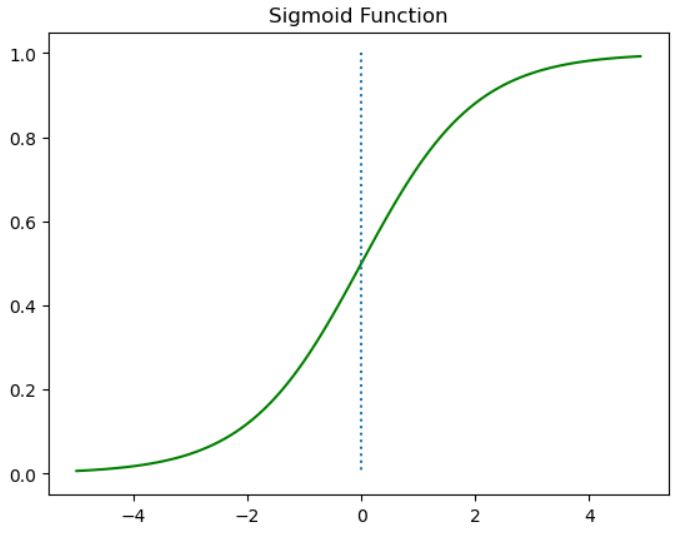
- w의 값에 따라 경사도가 변한다 (선형회귀에서 w가 직선에 기울기를 의미하는 것과 동일)
x = np.arange(-5.0, 5.0, 0.1)
y1 = sigmoid(0.5 * x) # x에 0.5의 가중치를 줌
y2 = sigmoid(x)
y3 = sigmoid(2 * x)

plt.plot(x, y1, 'r--', label='w:0.5')  # w의 값이 0.5일 때
plt.plot(x, y2, 'g', label='w:1')    # w의 값이 1일 때
plt.plot(x, y3, 'b--', label='w:2')  # w의 값이 2일 때
plt.legend() # 범례 표시
plt.plot([0, 0], [1.0, 0.0], ':') # 가운데 점선 표시
plt.title('Sigmoid Function')
plt.show()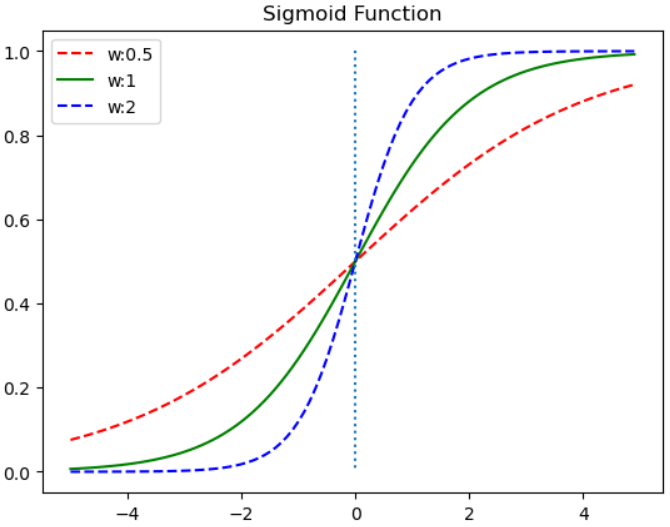
▶ 유방암 판별 예측
from sklearn.datasets import load_breast_cancer
from sklearn.linear_model import LogisticRegression
from sklearn.preprocessing import StandardScaler
# 정확도, 정밀도, 재현율, 혼동행렬
from sklearn.metrics import accuracy_score, precision_score, recall_score, roc_curve, roc_auc_score, confusion_matrix
from sklearn.model_selection import train_test_split
import pandas as pd
breast = load_breast_cancer()
print(breast.DESCR)df = pd.DataFrame(breast.data, columns=breast.feature_names)
df['target'] = breast.target
print(df.shape) # (569, 31)
display(df.head()) # (5, 31)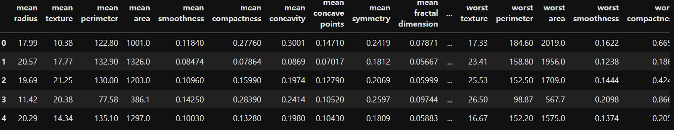
print(df['target'].value_counts()) # 악성종양 1, 양성종양 0
df.isna().sum() # 결측지 없음
df.describe() # (8, 31)
target
1 357
0 212
Name: count, dtype: int64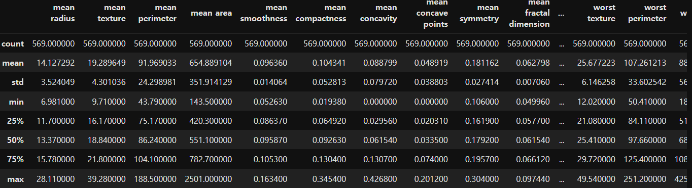
data_x = breast.data
data_y = breast.target
# 데이터 스케일링
scaled_data = StandardScaler().fit_transform(data_x)x_train, x_test, y_train, y_test = train_test_split(scaled_data, data_y, test_size=0.3, random_state=0, stratify=data_y)
# stratify : 종속변수의 분포가 학습과 평가 데이터에 같은 비율로 들어감
<회귀계수 최적화 옵션>
- solver : 최적화 문제에 사용될 알고리즘
- 'lbfgs' : 기본값, CPU 코어 수가 많다면 최적화를 병렬로 수행
- 'liblinear' : 작은 데이터에 적합한 알고리즘
- 'sag', 'saga' : 확률적 경사 하강법을 기반으로 한 알고리즘, 대용향 데이터에 적합
- 'newton-cg', 'sag', 'saga', 'lbfgs'만 다항 손실을 처리 -> 멀티클래스 분류 모델에 사용
- solver에 따른 규제 지원 사항
- newton-cg, lbfgs, sag : L2
- liblinear, saga : L1, L2
- multi-class : 다중 클래스 분류 문제의 상황에서 어떤 접근방식을 취할지 결정
- 'ovr' : 이진분류기인 sigmoid 함수를 이용해 결과 예측
- 'mutinomial' : softmax 확률값으로 다중 분류 수행
- C : 규제의 강도의 역수, C값이 작을수록 모델이 단순해진다 (=규제 강도가 강해진다)
- max_iter : solver가 결과를 수행하는데 필요한 반복횟수 지정 (default: 100)
# 모델 생성
model = LogisticRegression()
model.fit(x_train, y_train) # 학습

# 독립변수의 가중치
print('추정계수(가중치):', model.coef_)
print('절편:', model.intercept_)
추정계수(가중치): [[-0.54406091 -0.41605507 -0.51991133 -0.59308816 0.0027904 0.41939012
-0.78884789 -1.02290774 -0.15221315 0.37699245 -1.07237296 -0.06165012
-0.54319278 -0.69191037 -0.21537603 0.61125449 0.11034357 -0.26876198
0.49779553 0.42281321 -0.97636344 -1.08977767 -0.82614726 -0.86970513
-0.55575019 -0.15928048 -0.62816926 -0.7691139 -0.67505294 -0.73082045]]
절편: [0.23582794]
y_hat = model.predict(x_test)
# 앞에 20개의 정답과 예측
print('정답:', y_test[:20])
print('예측:', y_hat[:20])
정답: [0 0 0 1 0 1 0 0 0 0 0 1 1 1 0 0 0 1 0 0]
예측: [0 1 0 1 0 1 0 0 0 0 1 1 1 1 0 0 0 1 0 0]
<Confusion Matrix>
- 혼동행렬 함수는 행을 True, 열을 predict 값으로 이용
- 음성과 양성의 구분은 별도의 레이블을 지정하지 않으면 레이블 값의 정렬된 순서로 사용 (0:Negative, 1:Positive)
predict
--------------
N | P
--------------
|N| TN | FP |
true|-|---------|
|P| FN | TP |
--------------
matrix = confusion_matrix(y_test, y_hat)
print(matrix)
# 행이 실제 상황 / 열이 예측 상황
# 61 TN, 3 FP, 4 FN, 103 TP
[[ 61 3]
[ 4 103]]
# 평가지표

# (61 + 103) / (61 + 3 + 4 + 103) = 0.96
print(f'정확도: {accuracy_score(y_test, y_hat):.2f}')

# 103 / (3 + 103) = 0.97
print(f'정밀도: {precision_score(y_test, y_hat):.2f}')

# 103 / (4 + 103) = 0.96
print(f'재현율: {recall_score(y_test, y_hat):.2f}')
정확도: 0.96
정밀도: 0.97
재현율: 0.96
# positive라고 예측한 확률값
pred_proba_positive = model.predict_proba(x_test)[:,1]
# print(pred_proba_positive)
# 첫 번째 열은 negative로 예측할 확률, 두 번째 열은 positive로 예측할 확률 (0.5보다 크면 positive)

# roc_curve(정답, positive라고 예측한 확률값)
fpr, tpr, thresholds = roc_curve(y_test, pred_proba_positive)

# fpr, tpr, thresholds 3개의 값을 열로 변환해서 데이터프레임 생성
roc_data = pd.DataFrame(np.concatenate([fpr.reshape(-1,1), tpr.reshape(-1,1), np.round(thresholds.reshape(-1,1), 3)], axis=1), columns=['FPR', 'TPR', 'THRESHOLDS'])
display(roc_data)
# 임계값 변화에 따른 FPR 거짓양성율과 TPR 참양성율
print(f'AUC: {roc_auc_score(y_test, pred_proba_positive):.3f}')
# AUC: 0.99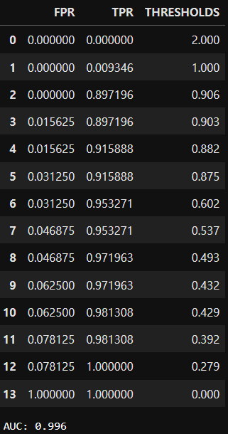
import matplotlib.pyplot as plt

plt.plot(fpr, tpr)
plt.xlabel('FPR')
plt.ylabel('TPR')
plt.show()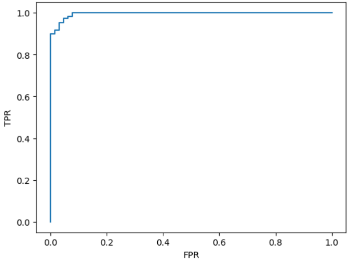
# 임계값 변화에 따른 재현율과 정밀도 변화 확인

# 실제 양성을 양성이라고 판단한 비율(TPR)과 음성을 양성이라고 잘못 판단한 위양성율(FPR)의 차이가 가장 큰 경우의 최적의 임계값
optimal_threshold = thresholds[np.argmax(tpr-fpr)]
print(f'최적의 임계값: {optimal_threshold:.3f}')
최적의 임계값: 0.493
from sklearn.metrics import classification_report

def threshold_filter(prob, threshold): # 확률값, 임계값
    return np.where(prob > threshold, 1, 0)

# 첫 번째 예측값 (양성으로 예측한 확률값, 임계값)
pred_1 = threshold_filter(pred_proba_positive, 0.5)

# 두 번째 예측값
pred_2 = threshold_filter(pred_proba_positive, 0.7)

# 세 번째 예측값
pred_3 = threshold_filter(pred_proba_positive, 0.3)

print(classification_report(y_test, pred_1))
print('='*60)
print(classification_report(y_test, pred_2))
print('='*60)
print(classification_report(y_test, pred_3))
precision recall f1-score support
0 0.94 0.95 0.95 64
1 0.97 0.96 0.97 107
accuracy 0.96 171
macro avg 0.96 0.96 0.96 171
weighted avg 0.96 0.96 0.96 171
============================================================
precision recall f1-score support
0 0.91 0.97 0.94 64
1 0.98 0.94 0.96 107
accuracy 0.95 171
macro avg 0.95 0.96 0.95 171
weighted avg 0.95 0.95 0.95 171
============================================================
precision recall f1-score support
0 0.97 0.92 0.94 64
1 0.95 0.98 0.97 107
accuracy 0.96 171
macro avg 0.96 0.95 0.96 171
weighted avg 0.96 0.96 0.96 171
# solver별 성능평가 비교
solvers = ['lbfgs', 'liblinear', 'newton-cg', 'sag', 'saga']

for solver in solvers:
    model = LogisticRegression(solver=solver, max_iter=600)
    model.fit(x_train, y_train)
    y_hat = model.predict(x_test)
    pred_proba_positive = model.predict_proba(x_test)[:,1]

    print(f'solver: {solver}, accuracy: {accuracy_score(y_test, y_hat):.3f}, auc: {roc_auc_score(y_test, pred_proba_positive):.3f}')
solver: lbfgs, accuracy: 0.959, auc: 0.996
solver: liblinear, accuracy: 0.959, auc: 0.996
solver: newton-cg, accuracy: 0.959, auc: 0.996
solver: sag, accuracy: 0.959, auc: 0.996
solver: saga, accuracy: 0.959, auc: 0.996
▶ 개인 신용도를 기반으로 대출 가능여부 예측
from sklearn.datasets import load_breast_cancer
from sklearn.linear_model import LogisticRegression
from sklearn.preprocessing import StandardScaler
from sklearn.metrics import accuracy_score, precision_score, recall_score, roc_curve, roc_auc_score, confusion_matrix
from sklearn.model_selection import train_test_split
import pandas as pd
df = pd.read_csv('./Dataset/Personal_Loan.csv')
print(df.shape) # (5000, 14)
display(df.head())
# 데이터 전처리
df.drop(['ID', 'ZIP Code'], axis=1, inplace=True)
df.head()
data_x = df.drop('Personal Loan', axis=1)
data_y = df['Personal Loan'].values
x_train, x_test, y_train, y_test = train_test_split(data_x, data_y, test_size=0.3, random_state=0, stratify=data_y)# 지수표현식에서 소수점 이하 3자리까지 출력
np.set_printoptions(precision=3, suppress=True)model = LogisticRegression(max_iter=2000)
model.fit(x_train, y_train)
coef = model.coef_.squeeze(axis=0) # 1차원 벡터의 형태로 변환
print('추정계수(가중치):', coef)
# 회귀계수 해석
# 로지스틱 회귀계수는 지수변환 exp()을 해주면 odds비가 나온다. odds비 = 성공확률 / 실패확률
odds_rate = np.exp(model.coef_).squeeze(axis=0)
coef_df = pd.DataFrame({'가중치':coef, 'odds비':odds_rate}, index=data_x.columns)
coef_df
# odds비 값이 높을수록 대출승인 확률이 높다추정계수(가중치): [-0.054 0.064 0.054 0.676 0.105 1.688 -0. -0.728 3.265 -0.553 -0.98 ]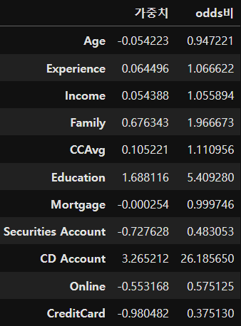
df['Education'].unique()
# array([1, 2, 3], dtype=int64)
# 대출거부 됐던 사람들의 교육수준의 평균값
print(df[df['Personal Loan'] == 0]['Education'].mean())
# 대출승인 됐던 사람들의 교육수준의 평균값
print(df[df['Personal Loan'] == 1]['Education'].mean())1.8435840707964601
2.2333333333333334
# 대출거부 됐던 사람들의 소득의 평균값
print(df[df['Personal Loan'] == 0]['Income'].mean())
# 대출승인 됐던 사람들의 소득의 평균값
print(df[df['Personal Loan'] == 1]['Income'].mean())
66.23738938053097
144.74583333333334
# 모델 예측 및 성능 측정
y_hat = model.predict(x_test)
print('정답:', y_test[:20])
print('예측:', y_hat[:20])

cf = confusion_matrix(y_test, y_hat)
cf_df = pd.DataFrame(cf, index=[['actual', 'actual'], ['대출불허(0)', '대출승인(1)']], # 멀티인덱스 지정
                     columns=[['predict', 'predict'], ['대출불허(0)', '대출승인(1)']])
display(cf_df)

print(f'정확도: {accuracy_score(y_test, y_hat):.3f}')
print(f'정밀도: {precision_score(y_test, y_hat):.3f}')
정답: [1 0 0 1 0 0 0 0 0 0 0 1 0 0 0 0 1 1 0 0]
예측: [1 0 0 0 0 0 0 0 0 0 0 1 0 0 0 0 0 1 0 0]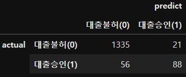
정확도: 0.949
정밀도: 0.807
pred_proba_positive = model.predict_proba(x_test)[:,1]
fpr, tpr, thresholds = roc_curve(y_test, pred_proba_positive)

plt.plot(fpr, tpr)
plt.xlabel('False Positive Rate')
plt.ylabel('True Positive Rate')
plt.show()

print(f'AUC: {roc_auc_score(y_test, pred_proba_positive):.3f}')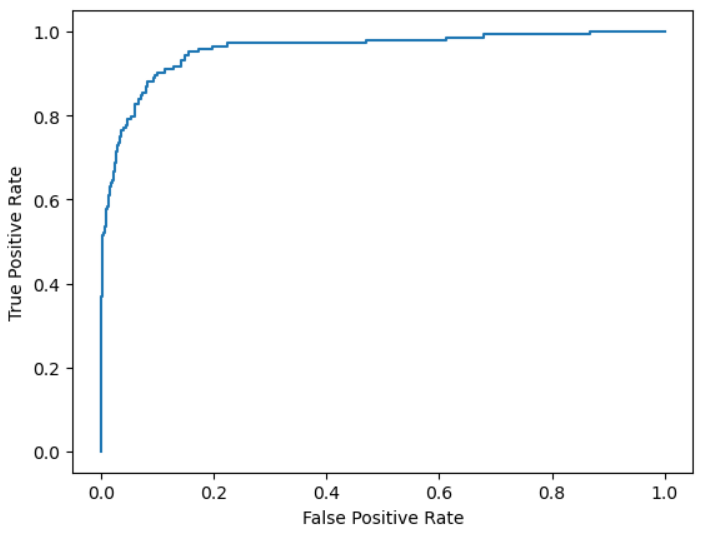
# 교차검증 (과적합 여부 확인)
from sklearn.model_selection import cross_validate

# 10번의 교차검증 수행
scores = cross_validate(model, data_x, data_y, cv=10, scoring=['accuracy', 'precision', 'roc_auc'])
for key, value in scores.items():
    print('평가지표:', key)
    print(f'평균값: {np.mean(value):.3f}')
    print('-'*30)
평가지표: fit_time
평균값: 0.252
------------------------------
평가지표: score_time
평균값: 0.003
------------------------------
평가지표: test_accuracy
평균값: 0.950
------------------------------
평가지표: test_precision
평균값: 0.810
------------------------------
평가지표: test_roc_auc
평균값: 0.958
------------------------------# 정확도: 0.949
평가지표: test_accuracy
평균값: 0.950
# 정밀도: 0.807
평가지표: test_precision
평균값: 0.810
# AUC: 0.956
평가지표: test_roc_auc
평균값: 0.958'데이터 분석 > 머신러닝' 카테고리의 다른 글
| [ML] 지도학습 알고리즘 - 다지분류, 다중 클래스 혼동행렬 (0) | 2023.11.21 |
|---|---|
| [ML] 지도학습 알고리즘 - 비용함수, 평가지표 (0) | 2023.11.21 |
| [ML] 4. 교차 검증 (Cross Validation) (1) | 2023.11.20 |
| [ML] 3. 규제 (Regulation) (0) | 2023.11.20 |
| [ML] 지도학습 알고리즘 - 분류분석, 다항 로지스틱 회귀분석 (0) | 2023.11.20 |