▶ Bagging - Regressor
- 보스톤 집값 예측
from sklearn.model_selection import train_test_split
from sklearn.ensemble import RandomForestRegressor
from sklearn.preprocessing import StandardScaler
from sklearn.metrics import mean_squared_error, r2_score
import pandas as pd
import numpy as np
# 데이터 로딩
boston = pd.read_csv('./Dataset/HousingData.csv')
boston.head()
# 결측치 제거
boston.dropna(inplace=True)
x = boston.drop('MEDV', axis=1)
y = boston['MEDV']# 학습, 평가 데이터 분할 및 스케일링
scaled_x = StandardScaler().fit_transform(x) # 표준화
x_train, x_test, y_train, y_test = train_test_split(scaled_x, y, test_size=0.3, random_state=10)# 모델 생성 및 검증
model = RandomForestRegressor(n_estimators=150, random_state=0) # 150개의 의사결정 나무를 만든다
model.fit(x_train, y_train)y_hat = model.predict(x_test)
print(f'RMSE: {np.sqrt(mean_squared_error(y_test, y_hat)):.3f}')
print(f'R2 ScoreL {r2_score(y_test, y_hat):.3f}')RMSE: 2.290
R2 ScoreL 0.906
# GridSearchCV를 이용한 파라미터 튜닝
from sklearn.model_selection import GridSearchCV

params = {'n_estimators':[10, 20, 50, 100, 200, 250],
          'max_features':[2, 4, 6, 8, 10],
          'bootstrap':[True, False]}  # True 복원 추출, False 비복원 추출
model = RandomForestRegressor()
gs = GridSearchCV(model, params, cv=5, scoring='neg_mean_squared_error')
gs.fit(scaled_x, y)

print('Best parameters:', gs.best_params_)
Best parameters: {'bootstrap': False, 'max_features': 4, 'n_estimators': 20}
y_hat = gs.best_estimator_.predict(x_test)
print(f'RMSE: {np.sqrt(mean_squared_error(y_test, y_hat)):.3f}')
print(f'R2 ScoreL {r2_score(y_test, y_hat):.3f}')
RMSE: 0.000
R2 ScoreL 1.000
# 최적화된 모형 저장
import pickle

with open('model.dat', 'wb') as f:
    pickle.dump(gs.best_estimator_, f)
print('모델 저장 완료')
import os
if os.path.exists('model.dat'):
with open('model.dat', 'rb') as f:
loaded_model = pickle.load(f)
y_hat = loaded_model.predict(x_test)
print(y_hat[:10])
# [29.6 23.7 37.3 13.1 25. 21.7 12.7 20.8 13.3 17.5]
▶ Bagging - Classifier
- 와인 품종 분류
from sklearn.ensemble import RandomForestClassifier
from sklearn.datasets import load_wine
from sklearn.metrics import confusion_matrix, classification_report, accuracy_score
# 데이터 로딩 및 확인
wine = load_wine()
print(wine.DESCR)**Data Set Characteristics:**
:Number of Instances: 178
:Number of Attributes: 13 numeric, predictive attributes and the class
:Attribute Information:
- Alcohol
- Malic acid
- Ash
- Alcalinity of ash
- Magnesium
- Total phenols
- Flavanoids
- Nonflavanoid phenols
- Proanthocyanins
- Color intensity
- Hue
- OD280/OD315 of diluted wines
- Proline
- class:
- class_0
- class_1
- class_2
x = wine.data
y = wine.target
df = pd.DataFrame(x, columns=wine.feature_names)
df['class'] = y
df.head()
print(df['class'].value_counts())
class
1 71
0 59
2 48
Name: count, dtype: int64
# 데이터 스케일링 및 분할
scaled_x = StandardScaler().fit_transform(x)
x_train, x_test, y_train, y_test = train_test_split(scaled_x, y, test_size=0.3, random_state=10, stratify=y)
# 모델 생성
model = RandomForestClassifier()
model.fit(x_train, y_train)# 모델 평가
y_hat = model.predict(x_test)
con_mat = confusion_matrix(y_test, y_hat)
print(con_mat)
report = classification_report(y_test, y_hat)
print(report)[[17 1 0]
[ 0 21 0]
[ 0 0 15]]
precision recall f1-score support
0 1.00 0.94 0.97 18
1 0.95 1.00 0.98 21
2 1.00 1.00 1.00 15
accuracy 0.98 54
macro avg 0.98 0.98 0.98 54
weighted avg 0.98 0.98 0.98 54
## 트리 시각화 ##
wine.target_names
# array(['class_0', 'class_1', 'class_2'], dtype='<U7')
from sklearn.tree import export_graphviz
estimator = model.estimators_[2] # 3번째 의사결정나무를 가져옴
#print(len(estimator)) 전체 100개
export_graphviz(estimator, out_file='tree.dot',
class_names=wine.target_names,
feature_names=wine.feature_names,
# max_depth=3, # 표현하고 싶은 최대 나무 깊이
precision=3, # 소수점 정밀도
filled=True, # 클래스별 색깔 채우기
rounded=True) # 박스 모양을 둥글게
<graphviz 패키지 설치>
- anaconda prompt 실행
- conda install python-graphviz
- 주피터랩 재기동
# flovanoids <= -0.797 : 자식 노드를 만들기 위한 규칙 조건
# gini : 불순도 (얾마나 다양한 클래스의 샘플들이 섞여있는지 나타내는 계수), 최종 지니 계수는 0
# samples : 현 노드의 규칙에 해당하는 데이터의 수
# value : 각 클래스에 해당하는 데이터의 수
# class : value값 중 다수의 값을 갖는 클래스 (해당 클래스로 분류가 된다는 의미)

import graphviz

with open('tree.dot') as f:
    tree = f.read()
graphviz.Source(tree)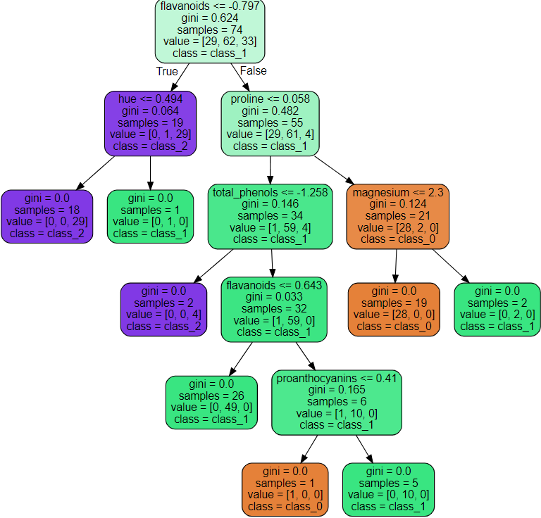
## 하이퍼 파라미터 튜닝 ##
from sklearn.model_selection import GridSearchCV

params = {'max_depth':[3, 4, 5, 6, 10], 'min_samples_split':[3, 6, 9, 10, 20, 30]}

# refit=True : 가장 좋은 파라미터 설정으로 재학습한 후 모델을 best_estimator_에 저장 (default)
gs = GridSearchCV(model, params, scoring='accuracy', cv=5)
gs.fit(x, y)
print('최적 파라미터:', gs.best_params_)
print(f'최적 파라미터 정확도: {gs.best_score_:.3f}')최적 파라미터: {'max_depth': 3, 'min_samples_split': 20}
최적 파라미터 정확도: 0.983
Feature Importance
- 의사결정 나무 알고리즘이 학습을 통해 규칙을 정하는데 있어 피처의 중요한 역할지표를 제공하는 속성
- 일반적으로 값이 높을수록 해당 피처의 중요도가 높다는 의미로 해석
im = gs.best_estimator_.feature_importances_importance = {k:v for k, v in zip(wine.feature_names, im)}
df_importance = pd.DataFrame(pd.Series(importance), columns=['importance'])
df_importance = df_importance.sort_values('importance', ascending=False)
df_importance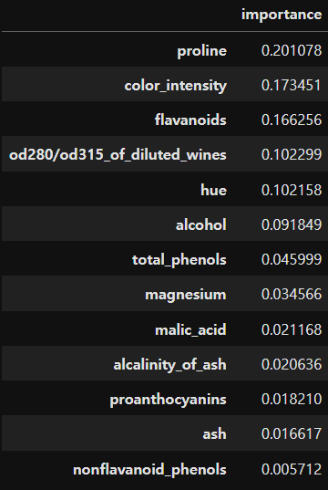
import seaborn as sns
import matplotlib.pyplot as plt

sns.barplot(df_importance, x='importance', y=df_importance.index)
plt.show()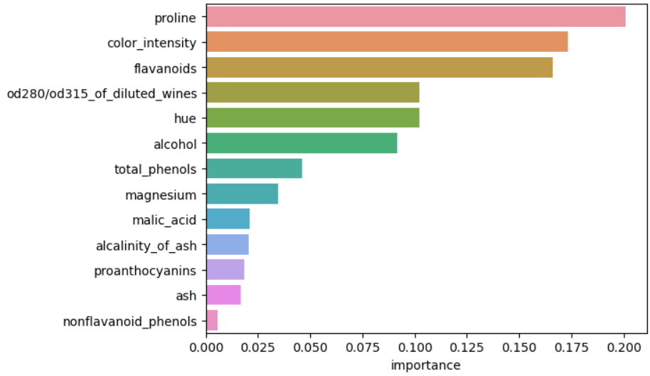
'데이터 분석 > 머신러닝' 카테고리의 다른 글
| [ML] 10. 앙상블 - Boosting (0) | 2023.11.23 |
|---|---|
| [ML] 9. 앙상블 - Voting (0) | 2023.11.23 |
| [ML] 7. KNN (0) | 2023.11.22 |
| [ML] 6. 나이브 베이즈 (0) | 2023.11.22 |
| [ML] 지도학습 알고리즘 - 앙상블 러닝 (0) | 2023.11.22 |