[ML] 2. 데이터 전처리

▶ One-hot Encoding
- 입력 값으로 2차원 데이터가 필요하다.
- 인코딩 결과가 밀집행렬(Dense matrix)이기 때문에 다시 희소행렬(Parse matrix)로 변환해야 한다.
 

from sklearn.preprocessing import OneHotEncoder
import numpy as np

maker = ['Samsung', 'LG', 'Apple', 'SK']
maker = np.array(maker).reshape(-1,1) # 1차원 벡터를 2차원 행렬로 변환
print(maker)

encoder = OneHotEncoder()
encoder.fit(maker)
one_hot = encoder.transform(maker) # transform : 변환하고자하는 데이터를 넣어줌

print('원-핫 인코딩 결과(밀집행렬)')
print(one_hot)
print()
print('원-핫 인코딩 결과(희소행렬)')
print(one_hot.toarray()) # 배열로 변환

[['Samsung']
 ['LG']
 ['Apple']
 ['SK']]
원-핫 인코딩 결과(밀집행렬)
  (0, 3)	1.0
  (1, 1)	1.0
  (2, 0)	1.0
  (3, 2)	1.0

원-핫 인코딩 결과(희소행렬)
[[0. 0. 0. 1.]
 [0. 1. 0. 0.]
 [1. 0. 0. 0.]
 [0. 0. 1. 0.]]

 
   
   ▷ OneHotEncoder 데이터프레임에 적용
 

import pandas as pd

df = pd.DataFrame({'maker':['Samsung', 'LG', 'Apple', 'SK']})
encoder = OneHotEncoder()
encoded = encoder.fit_transform(df['maker'].values.reshape(-1,1)).toarray().astype(int) # 준비와 실제 변환을 동시에 수행
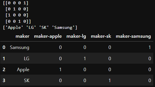
print(encoded)
print(np.sort(df['maker']))
df[['maker-apple', 'maker-lg', 'maker-sk', 'maker-samsung']] = encoded
df

 

 

import pandas as pd

df = pd.DataFrame({'maker':['Samsung', 'LG', 'Apple', 'SK']})
pd.get_dummies(df, columns=['maker'])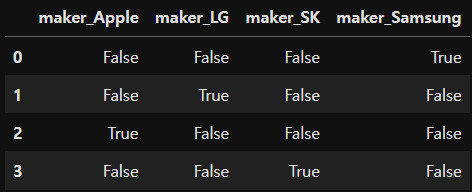

---

 
▶ Label Encoding
 

from sklearn.preprocessing import LabelEncoder

language = ['Java','Python','C#','Pascal']
df = pd.DataFrame({'Language': language})
print('라벨 인코딩 전')
display(df)
encoded = LabelEncoder().fit_transform(language)
# print(encoded)
df['language'] = encoded
print('라벨 인코딩 후')
df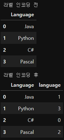

 

language = ['Java','Python','C#','Pascal']
df = pd.DataFrame({'language': language})

# language 값 정렬 (i는 인덱스, v는 값), v:i -> 값이 키가 되고 인덱스는 벨류
map_data = {v:i for i,v in enumerate(df['language'].sort_values())} 
df['language'] = df['language'].map(map_data)
df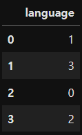

---

 
▶ 데이터 스케일링
 
    ▷ 표준화 (Standardization)
 

from sklearn.datasets import load_iris
import pandas as pd

iris = load_iris()
iris_df = pd.DataFrame(iris.data, columns=iris.feature_names)
# iris_df['target'] = iris.target # 정답
# print(iris_df['target'].unique()) # [0 1 2]
display(iris_df.head())

print('컬럼 평균')
print(iris_df.mean())

print('컬럼 분산')
print(iris_df.var())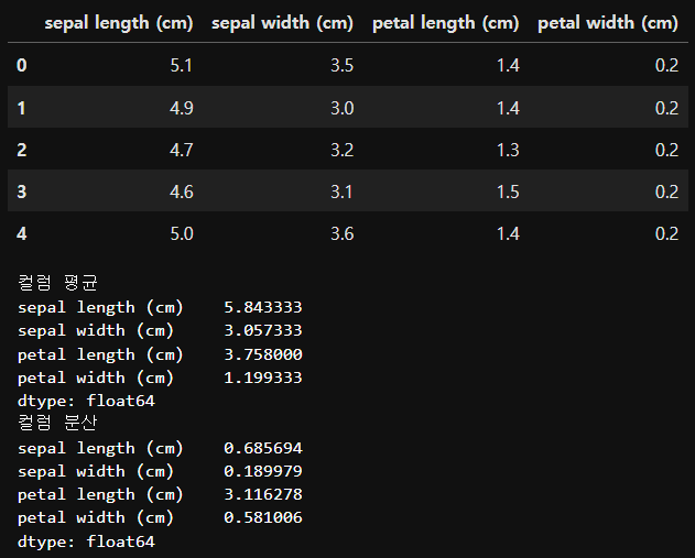

 

from sklearn.preprocessing import StandardScaler

scaler = StandardScaler()
scaler.fit(iris_df) 
iris_scaled = scaler.transform(iris_df)

# 또는 iris_scaled = scaler.fit_transform(iris_df)

iris_scaled_df = pd.DataFrame(iris_scaled, columns=iris.feature_names)
display(iris_scaled_df.head())

print('표준화된 컬럼 평균')
print(iris_scaled_df.mean())
# -1.690315e-15 : -1.69 * 10(-15승) 

print('표준화된 컬럼 분산')
print(iris_scaled_df.var())

print('표준화된 컬럼 표준편차')
print(iris_scaled_df.std())
# 평균은 0에 근사한 값, 표준편차는 1에 근사한 값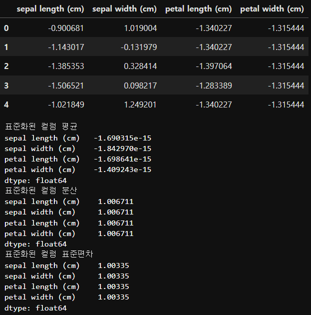

 
   
    ▷ 정규화 (Normalization)

from sklearn.preprocessing import MinMaxScaler

# 데이터를 0에서 1사이의 값으로 변환
iris_scaled = MinMaxScaler().fit_transform(iris_df)
iris_scaled_df = pd.DataFrame(iris_scaled, columns=iris.feature_names)
display(iris_scaled_df.head()) 

print('정규화된 컬럼 최소값')
print(iris_scaled_df.min())

print('정규화된 컬럼 최대값')
print(iris_scaled_df.max())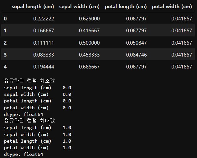

---

 
▶ 불균형 데이터 처리
 
    ▷ imbalanced-learn 모듈 설치
 

!pip install imbalanced-learn

!pip install imblearn

!pip install scikit-learn==1.2.2 --user

import numpy as np
import pandas as pd

from sklearn.datasets import make_classification
from collections import Counter

import matplotlib.pyplot as plt
import seaborn as sns

from imblearn.under_sampling import RandomUnderSampler, TomekLinks
from imblearn.over_sampling import RandomOverSampler, SMOTE

 
   
    ▷ 불균형 데이터 생성
 

x, y = make_classification(n_samples=10000, n_features=5, weights=[0.99], flip_y=0, random_state=10) 
# n_features는 독립변수(컬럼)의 개수, weights는 종속변수의 비율, y는 0과 1, random_state=10 seed값 고정
# flip_y : y값이 임의로 변경되는 비율 (default:0.01)

print(x[:2,:])
print(x.shape, y.shape) # x는 10000행 5열, y는 10000개
print(np.unique(y)) # [0 1]
print(Counter(y)) # {0: 9839, 1: 161}, flip_y = 0 지정하면 {0: 9900, 1: 100}

[[ 0.38201186 -0.10502417 -1.65203303 -0.0260045   0.80085356]
 [ 0.03174755  0.65503326  0.94612307  0.32881832 -0.80422025]]
(10000, 5) (10000,)
[0 1]
Counter({0: 9900, 1: 100})

 

# x는 3번째 컬럼, y는 4번째 컬럼
sns.scatterplot(x=x[:,3], y=x[:,4], hue=y)
plt.show()

 
 
▶ Under Sampling
 
    ▷ Random Under Sampling
 

# sampling_strategy='majority' : 다수 집단에서 언더 샘플링하여 소수 집단의 수와 동일하게 맞춘다
under_sample = RandomUnderSampler(sampling_strategy='majority')
x_under, y_under = under_sample.fit_resample(x, y)
print(Counter(y_under)) # 소수 집단의 1에 맞춰 100으로 맞춰줌

Counter({0: 100, 1: 100})

 

sns.scatterplot(x=x_under[:,3], y=x_under[:,4], hue=y_under)
plt.show()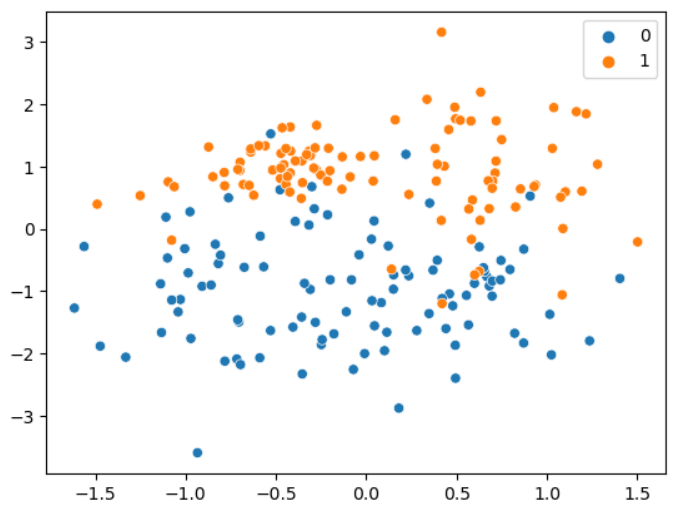

 

# sampling_strategy의 값을 0~1 사이의 값으로 지정하면 비율 값(소수집단 데이터수/다수집단 데이터 수)으로 다수 집단 데이터를 샘플링 한다. (0.4 = 100/250    250은 다수집단 수)
under_sample = RandomUnderSampler(sampling_strategy=0.4)
x_under, y_under = under_sample.fit_resample(x, y)
print(Counter(y_under)) # {0: 250, 1: 100}

Counter({0: 250, 1: 100})

 

sns.scatterplot(x=x_under[:,3], y=x_under[:,4], hue=y_under)
plt.show()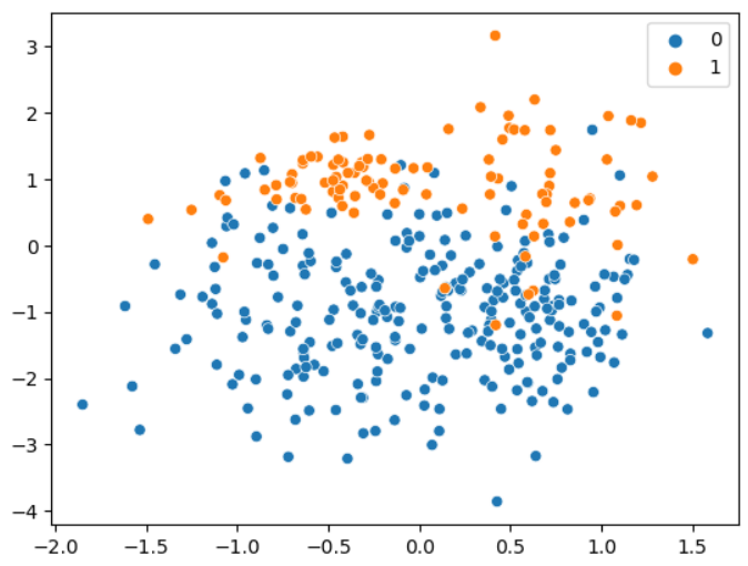

 
 
▶ Tomek Link
<sampling strategy>
  - majority : 다수의 집단 데이터만 샘플링
  - not minority : 소수 집단을 제외한 나머지 범주 데이터를 리샘플링
  - mot majority : 다수 집단을 제외한 나머지 범주 데이터를 리샘플링
  - all : 모든 범주 데이터를 리샘플링
  - auto : not minority와 동일
 

tomek_link = TomekLinks(sampling_strategy='auto')
x_under, y_under = tomek_link.fit_resample(x, y)
print(Counter(y_under)) # {0: 9854, 1: 100}

Counter({0: 9854, 1: 100})

 

sns.scatterplot(x=x_under[:,3], y=x_under[:,4], hue=y_under)
plt.show()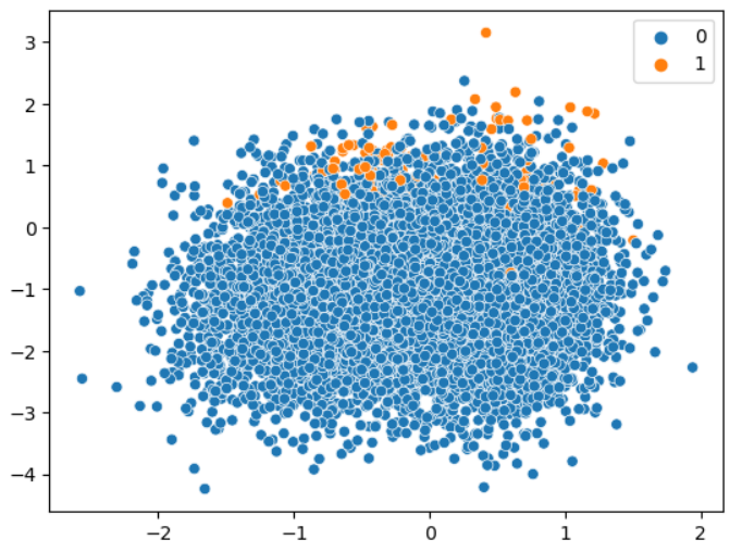

 
 
▶ Over Sampling
 
    ▷ Random Over Sampling
 

over_sample = RandomOverSampler(sampling_strategy='minority')
x_over, y_over = over_sample.fit_resample(x, y)
print(Counter(y_over)) # {0: 9900, 1: 9900}

Counter({0: 9900, 1: 9900})

 
 

# 동일 데이터에 대해 반복적으로 복제해서 만들었기 때문에 산점도가 원본 데이터와 같아 보인다
sns.scatterplot(x=x_over[:,3], y=x_over[:,4], hue=y_over)
plt.show()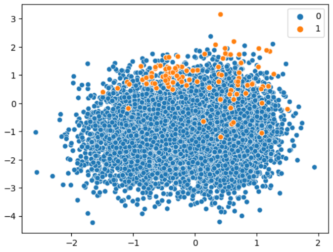

 
 
    ▷ SMOTE

smote_sample = SMOTE(sampling_strategy=0.4)
x_sm, y_sm = smote_sample.fit_resample(x, y)
print(Counter(y_sm)) # {0: 9900, 1: 3960}

Counter({0: 9900, 1: 3960})

 

sns.scatterplot(x=x_sm[:,3], y=x_sm[:,4], hue=y_sm)
plt.show()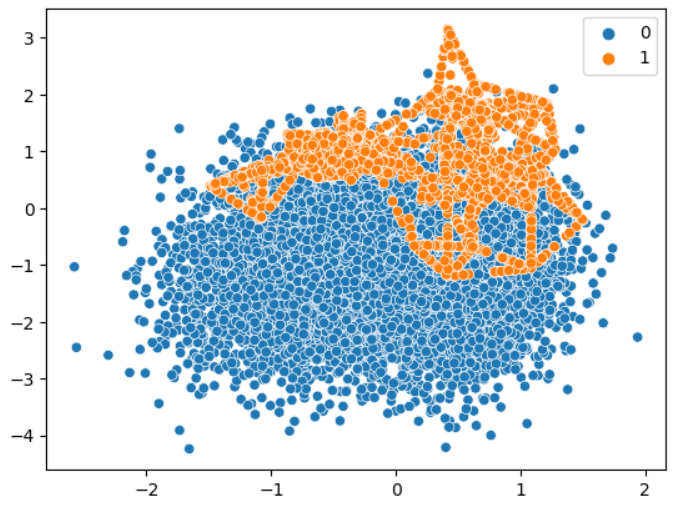

 
 
▶ Cost Sensitive Learning
- 라벨 가중치 옵션 사용
 

from sklearn.model_selection import RepeatedStratifiedKFold, cross_val_score # 교차검증, 평가점수
from sklearn.ensemble import RandomForestClassifier

def evaluate_model(x, y, model):
    cv = RepeatedStratifiedKFold(n_splits=5, n_repeats=3, random_state=1) # n_splits 5등분, 3회 반복
    scores = cross_val_score(model, x, y, scoring='precision', cv=cv, n_jobs=-1) # cv는 교차검증 객체,  n_jobs=-1 가동 가능한 모든 코어를 이용해서 교차검증을 수행
    return scores

model = RandomForestClassifier(n_estimators=100) # n_estimators 의사 결정나무 100개
scores = evaluate_model(x, y, model)
print(f'Mean Precision No weight: {np.mean(scores):.3f}') # 가중치를 주지 않은 상태에서의 평균 정밀도

# class_weight: 종속변수 label별 가중치
# balanced: 각 클래스에 대해 [전체 샘플 수/(클래스 수 * 클래스별 빈도)]로 계산된 가중치 부여
# 10000/(2*9900), 10000/(2*100)
weights = {0:1.0, 1:10} # 1대10 비율 가중치
model = RandomForestClassifier(n_estimators=100, class_weight=weights)#'balanced') # n_estimators 의사 결정나무 100개
scores = evaluate_model(x, y, model)
print(f'Mean Precision weight: {np.mean(scores):.3f}')

Mean Precision No weight: 0.292
Mean Precision weight: 0.329